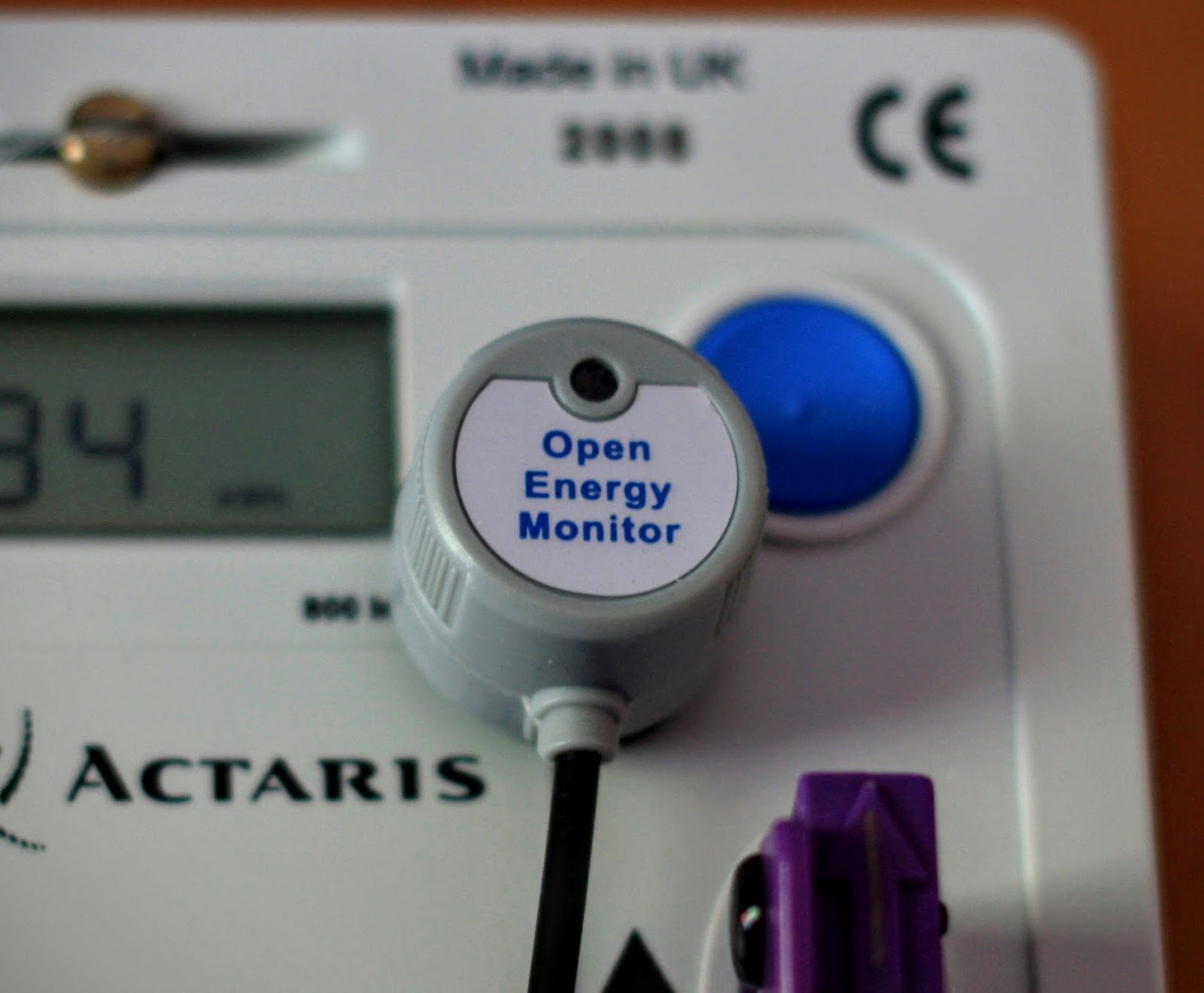
Optical Utility Meter LED Pulse Sensor attached to meter via removable sticky pad

We have just taken delivery of a batch of custom made Optical Utility Meter LED Pulse Sensor units. We're very excited about these new sensors, they will enable the emonPi and emonTx to interface directly with Utility Meters measuring exactly the amount of energy being measured by the utility meter.

The Optical Pulse Sensor works by sensing the LED pulse output from utility meters. Each pulse corresponds to a certain amount of energy passing through the meter. The amount of energy each pulse corresponds to depends on the meter. By counting these pulses the meters KWh value can be calculated.

Unlike clip-on CT based monitoring pulse counting is measuring exactly what the utility meter is measuring i.e. what you get billed for. The pulse counting cannot provide an instantaneous power reading like CT based can. Where possible we recommend using pulse counting in conjunction with CT monitoring. The emonPi and emonTx can simultaneously perform pulse counting and CT based monitoring.

In the future we plan to look at how the pulse counting energy value can be used to calibrate the CT based power calculations.

The Optical Pulse sensor will work plug-and-play with emonPi / emonTx connecting via RJ45 socket, older units will require a firmware update. See documentation page for update instructions.

Optical Pulse Sensor Documentation Page

Optical Pulse Sensor is now available to purchase from the OpenEnergyMonitor online shop

If you have backed us on Kickstarter or have purchased an emonPi from us as a thank you for your support we would like to offer you 20% off the Optical Pulse Sensor, use code PYN5031978E9T at checkout (valid until 1st July 2015).

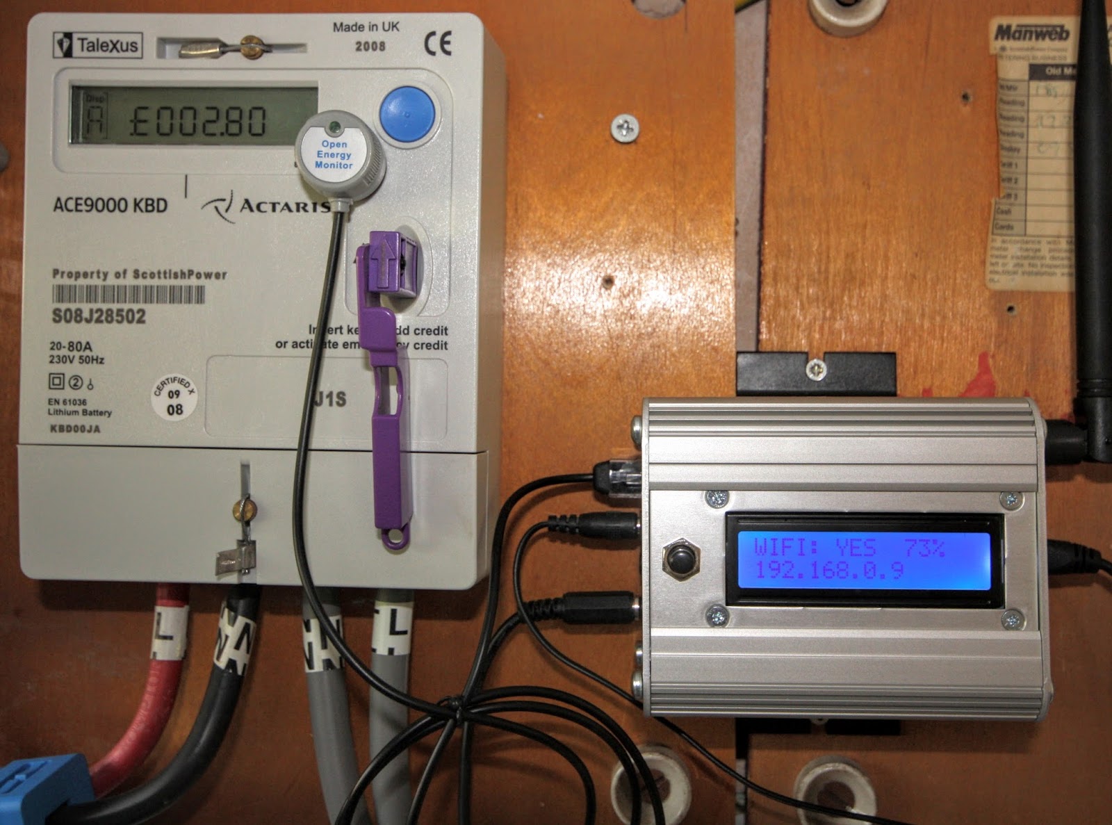
Pulse sensor installed & connected to emonPi via RJ45

Big box of pulse sensors arrived today! :-)

We hear a lot that a renewable energy system benefits from having a mix of generating technologies. Combining wind and solar for example is said to provide a higher supply/demand matching than relying on one technology alone. When the wind isn’t blowing it may be sunny or vice versa.
How do we work out the best mix of different renewable generating technologies. When is it cheaper to add more wind than to add more solar, what is the balance point for a particular demand profile?

This example explore's the balance point for onshore wind + solar, both having large resource availabilities associated with them. The mix will be balanced based on energy cost. It would also be good to explore the balance based on embodied energy. As with all modelling based on costs the outcome will change as costs change, the important thing here is to understand the method so that we can explore for a given set of costs what the optimum mix might be.
In the recent contracts for a difference auction in the UK for renewable generation many of the onshore wind farms received a strike price of £82.50 per MWh. Two offshore wind projects received £115 per MWh and three solar farms received £79.23 per MWh.
Source: Contracts for Difference Auction Results

In this example we will use these cost figures, the ZCB capacity dataset for onshore wind and solar and a simple flat demand profile.

If we look at the results from example 2 investigating annual matching for wind and solar and add in the cost information:

• 1.164kW of onshore wind delivers 3300 kWh/y at £272/y and a supply/demand matching of 65.88%.
• 3.99kW of solar delivers 3300 kWh/y at £261/y and a supply/demand matching of 40.61%.

One way to investigate the best mix is to fix the total annual energy cost and change the installed capacities of both solar and wind to achieve the greatest level of matching for a given energy cost.

So lets take an annual energy cost of £272 and work out for this cost what is the maximum level of matching we can obtain from a wind + solar mix.


Online tool: http://openenergymonitor.org/energymodel > navigate to 4. Mixed supply and flat demand

Cost	Wind capacity	Solar capacity	Matching
£272.02	1.1635	0	65.86 %
£272.03	1.0235	0.5	70.04 %
£272.03	0.9395	0.8	71.22 %
£272.03	0.9115	0.9	71.33%
£272.04	0.8975	0.95	71.35%
£272.04	0.8835	1.0	71.34 %
£272.04	0.8695	1.05	71.31 %
£272.04	0.8555	1.1	71.26 %
£272.04	0.8275	1.2	71.09%

At an energy cost of £272/year a flat demand and the ZCB dataset we can see a clear benefit from combining solar and wind in the energy mix, increasing solar pv capacity appears to make sense up to 105.8% of installed wind capacity after which the matching starts to drop again for the given energy cost.

Its important to note however that wind still provides the majority of the electricity at 2543 kWh of the 3300 kWh generated annually (76%). This is because of wind's higher capacity factor in comparison with solar.

How does the mix change if we decide to oversupply and pay a higher cost for the electricity. If we fix our annual cost to say £320

Cost	Wind capacity	Solar capacity	Matching
£320.06	1.369	0	69.88 %
£320.07	1.229	0.5	73.98 %
£320.08	1.144	0.8	75.20 %
£320.08	1.089	1.0	75.44 %
£320.08	1.075	1.05	75.45 %
£320.08	1.061	1.1	75.44 %
£320.08	1.047	1.15	75.41 %
£320.08	1.033	1.2	75.37 %

The maximum matching we obtained in this case happened where solar capacity was 97.7% of wind capacity.

It appears that in these model runs, the optimal mix between solar and wind is to install an equal capacity of both, its interesting that this happens to be the case and that its not say half the wind capacity. The model results confirm the often discussed complementarity between solar and wind supply and that the benefit of their combination increases supply demand matching by around 5% points for no additional cost and is a similar scale of supply/demand matching improvement seen by increasing the oversupply of wind to 120% of demand but without the additional cost.

Download python model:
http://openenergymonitor.org/energymodel/python/windandsun.py

The ZeroCarbonBritain dataset includes 10 years of hourly traditional electricity demand data for the UK. The previous example compared renewable supply data with a flat demand profile, this example explores the effect of the variable traditional electricity demand profile with its day time peaks and night time low on supply/demand matching for the different renewable energy generators.

The screenshot below gives a flavour for what the traditional electricity demand profile looks like in blue, the black line is the supply from onshore wind, using the tool you can compare traditional electricity demand to: onshore wind, offshore wind, tidal, wave and solar power.

Online tool: http://openenergymonitor.org/energymodel > navigate to 3. Variable supply, traditional electricity demand and oversupply

These are the results for the amount of demand supplied directly for each generation type, matching annual supply totals with demand totals:

	Onshore wind	Offshore wind	Wave	Tidal	Solar
Installed capacity	1.17kW	0.79kW	1.33kW	1.58kW	3.98kW
Percentage of demand supplied directly	66.5%	76.7%	75.2%	57.0%	42.1%
Percentage of time demand is more or the same as the supply	40.7%	46.5%	44.7%	38.7%	31.1%

Interestingly they only change marginally. Solar PV makes a gain 2% on the demand supplied directly which reflects higher demand in the day vs night time and we see a couple of other 1% changes but the differences are quite marginal and smaller than the difference between each renewable energy type so we don’t really see any change of order.

Increasing the degree of supply/demand matching between a variable renewable supply and traditional electricity demand by over supply

The are multiple ways of increasing the level of supply/demand matching or reducing the unmet demand. Over-supply is one way we can do this and is one of the measures used in the ZeroCarbonBritain scenario. In the previous examples we sized the installed capacity of the renewable electricity generating technologies to produce over the 10 year model period the exact same amount of electricity as was used in the 10 year period.
We can re-run the same model but with installed capacity amounts set to 110%, 120% or 130% of demand

Oversupply: 110%

	Onshore wind	Offshore wind	Wave	Tidal	Solar
Installed capacity	1.28kW	0.86kW	1.46kW	1.74kW	4.39kW
Percentage of demand supplied directly	68.9%	79.6%	77.9	58.9%	43.0%
Percentage of time demand is more or the same as the supply	44.1%	51.8%	50.0%	41.7%	32.4%

Oversupply: 120%

	Onshore wind	Offshore wind	Wave	Tidal	Solar
Installed capacity	1.28kW	0.94kW	1.60kW	1.89kW	4.79kW
Percentage of demand supplied directly	71.1%	81.9%	80.3%	60.4%	43.8%
Percentage of time demand is more or the same as the supply	47.2%	56.5%	54.3%	44.3%	33.5%

Oversupply: 130%

	Onshore wind	Offshore wind	Wave	Tidal	Solar
Installed capacity	1.51kW	1.02kW	1.73kW	2.05kW	5.19kW
Percentage of demand supplied directly	72.9%	83.9%	82.2%	61.7%	44.5%
Percentage of time demand is more or the same as the supply	50.1%	60.7%	58.1%	46.7%	34.4%

For every 10% of demand increase in supply we see 1-3% improvements in the percentage of demand supplied directly and 1-5% improvements in the amount of time demand is more or the same as supply.

The python code for the above examples is very similar to the previous example for the flat demand profile and can be downloaded here: http://openenergymonitor.org/energymodel/#python

The next example looks at the question of complementarity between different renewable energy types and asks the question what might the optimum capacity mix point be between wind and solar for a given electricity price point.

The second example in the hourly energy modelling tool models the degree of supply/demand matching between a variable renewable supply consisting of a single renewable energy generation type and a flat electricity demand profile.

A flat demand may not of course be particularly realistic and the more complex examples later on address this, but I've used it here just to illustrate this particular simple example case.



Online tool: http://openenergymonitor.org/energymodel > navigate to 2. variable supply and flat demand
 
The demand is subtracted from the supply for every hour in the 10 year period and the total amount of unmet demand and excess generation is measured as well as the amount of time the supply was more than or equal to the demand.

The demand level is set to an annual average electricity demand of 3300 kWh which is the average UK household annual electricity consumption. The amount of installed capacity is set to match this demand on the 10 year basis of the dataset.

Running the model for each of each generation type, matching total 10 year supply to total 10 year demand of 3300 kWh x 10 we get the following results:

	Onshore wind	Offshore wind	Wave	Tidal	Solar
Installed capacity	1.17kW	0.79kW	1.33kW	1.58kW	3.98kW
Percentage of demand supplied directly	65.9%	76.4%	73.9%	57.7%	40.6%
Percentage of time demand is more or the same as the supply	40.1%	46.2%	45.3%	38.6%	32.1%

We can see again here that offshore wind is the clear winner with the lowest installed capacity requirement and highest level of supply/demand matching. Perhaps an interesting result is how less predictable technologies such as wind and wave provide greater levels of matching than power from tidal which is very predictable.

Python example source code
Alongside the online javascript modelling tool there are a series of python versions of the examples which are simpler to follow as they dont include all the code to create the visual output, they just print out the main results at the end.

I've highlighted the main parts in bold below:

# dataset index:
# 0:onshore wind, 1:offshore wind, 2:wave, 3:tidal, 4:solar, 5:traditional electricity
gen_type = 1

installed_capacity = 0.785 # kW

annual_house_demand = 3300 # kWh
house_power = (annual_house_demand * 10.0) / 87648  

# Load dataset
with open("../dataset/tenyearsdata.csv") as f:
    content = f.readlines()
hours = len(content)

print "Total hours in dataset: "+str(hours)+" hours"
print

total_supply = 0
total_demand = 0

exess_generation = 0
unmet_demand = 0

hours_met = 0


# for every hour in the dataset
for hour in range(0, hours):
    values = content[hour].split(",")
    
    # calculate the supply
    supply = float(values[gen_type]) * installed_capacity
    total_supply += supply
    
    # calculate demand
    demand = house_power
    total_demand += demand
    
    # subtract demand from supply to find the balance
    balance = supply - demand
    
    # record the total amount of exess and unmet demand
    if balance>=0:
        exess_generation += balance
        hours_met += 1
    else:
        unmet_demand += -balance

capacity_factor = total_supply / (installed_capacity*hours) * 100

prc_demand_supplied = ((total_demand - unmet_demand) / total_demand) * 100

prc_time_met = (1.0 * hours_met / hours) * 100





# print out the results
print "Installed capacity: %s kW" % installed_capacity
print "Capacity factor: %d%%" % capacity_factor
print
print "Total supply: %d kWh" % total_supply
print "Total demand: %d kWh" % total_demand
print
print "Exess generation %d kWh" % exess_generation
print "Unmet demand %d kWh" % unmet_demand
print
print "Percentage of demand supplied directly %d%%" % prc_demand_supplied
print "Percentage of time supply was more or the same as the demand %d%%" % prc_time_met

This first example in the hourly energy modelling tool model's the hourly output of a given installed capacity of wind, wave, tidal or solar. The model really isn’t doing much its just loading the capacity factors for every hour from the 10 year dataset and multiplying the capacity factor by the installed capacity.

The total electricity generated is calculated as the sum of the electricity generation in each hour and printed along with the capacity factor at the end.

This example is useful for just seeing what the ZeroCarbonBritain renewable capacity factor dataset looks like, you can zoom and pan through the datasets for onshore wind, offshore wind, tidal, wave and solar pv, click on the link below to open the tool:
  
Online tool: http://openenergymonitor.org/energymodel > navigate to 1. variable supply

The units are really not important the example could just as well be in MW's or GW's. kW's where chosen as the other model examples in the series are focused around building a hourly model that's relatable to an average households energy demand. The kW's of installed capacity could just relate to a small share of a much larger wind turbine, solar farm, wave or tidal power installation.

Running the model for each of these generation types with the same installed capacity the results are as follows:

	Onshore wind	Offshore wind	Wave	Tidal	Solar
Installed capacity	1.0kW	1.0kW	1.0kW	1.0kW	1.0kW
Annual generation	2834 kWh	4204 kWh	2482 kWh	2092 kWh	826 kWh
Capacity factor	32%	47%	28%	23%	9%

In all of the examples above the installed capacity of the renewable generator was the same (1.0kW) but we can see straight away that there is a significant difference in the total electricity generated by each type. A unit of offshore wind generates just over 5 times as much energy as a unit of solar pv using the zerocarbonbritain dataset. By itself this is not enough information to evaluate the effectiveness of a technology, we would need to compare the costs per unit of installed capacity, embodied energy per unit of installed capacity, how well a particular solution matches demand, the land areas required, the availability of the resource to name just a few of the many factors that need to be weighed up but it does highlight one of the important factors.

Python example source code
Alongside the online javascript modelling tool there are a series of python versions of the examples which are simpler to follow as they dont include all the code to create the visual output, they just print out the main results at the end.

The following 19 lines of python code are all you need to load the ZeroCarbonBritain dataset and run through all 87,648 hours, calculating the power output for each hour and accumulating the total energy supplied over the 10 year model period:

# dataset index:
# 0:onshore wind, 1:offshore wind, 2:wave, 3:tidal, 4:solar, 5:traditional electricity
gen_type = 4

installed_capacity = 1.0 # kW

# Load dataset
with open("../dataset/tenyearsdata.csv") as f:
    content = f.readlines()
hours = len(content)

print "Total hours in dataset: "+str(hours)+" hours"

total_supply = 0

for hour in range(0, hours):
    values = content[hour].split(",")
   
    supply = float(values[gen_type]) * installed_capacity
    total_supply += supply

capacity_factor = total_supply / (installed_capacity*hours) * 100

print "Installed capacity: %s kW" % installed_capacity
print "Total supply: %d kWh" % total_supply
print "Capacity factor: %0.2f%%" % capacity_factor

Next: Variable supply and flat demand - investigating the degree of supply/demand matching

Earlier this year I did some work with Philip James from the Centre for Alternative Technology and a researcher on the ZeroCarbonBritain project on creating an open source online zero carbon energy modelling tool based on the ZeroCarbonBritain energy model which is one of the Uk's leading energy scenarios outlining a positive, aspirational 100% renewable zero carbon energy future.

This first tool is available online here and blog post, using it it is possible to explore how its possible to supply energy demands such as space heating and electric vehicles from a variable renewable supply consisting of wind, solar, tide and wave power and a mix of storage technologies. The tool models supply and demand on an hourly basis which is a significant improvement over simpler annual approach.

Understanding its workings
I had been wanting to dig down deeper into the workings of the model and unpick the effect of the different components, the full model has so many different things going on that its hard to see how each component such as space heating demand from heatpumps, space heating profiles, electric vehicle charging profiles, water heating, or different generation technologies affects the bigger picture of the overall supply/demand balance and resulting storage requirements and so over the last month and a half I've spent some time looking into this in more detail.

Python and javascript example models
I started by writing a series of python models that modelled many of the key components in turn using the full 10 year hourly dataset used in the ZeroCarbonBritain spreadsheet model, exploring the level of supply/demand matching for each generation technology. As I started to model some of the more complex demands such as space heating from heatpumps, including the effect of solar and internal gains, I needed to be able to see what was going on in more detail so I converted the models to javascript and wrote a data viewer using flot.

Online visual tool
I've put all these model examples together into an online tool and added alongside each model a brief analysis and extended results of the many model run's I ran with different parameters. The tool also includes an introduction and overview of the uk energy context which is intended to help put the model examples which focus on domestic traditional electricity demand, space heating and electric transport in context. This tool is now available online here:


Launch online zero carbon energy system example models: http://openenergymonitor.org/energymodel

and its all open source with the code and full website on github here:
https://github.com/TrystanLea/zcem

The tool covers the following model examples and context pages:

    Introduction
    Energy Overview
    1. Variable supply
    2. Variable supply and flat demand
    3. Variable supply, traditional electricity demand and oversupply
    4. Mixed supply and flat demand
    5. Variable supply and space heating demand
    6. Electric Vehicles
    7. All
    Aggregation
    ZCB Dataset
    ZCB web model
    Python models

I have found it really interesting doing this work, but it also feels like a chapter early on in a large book. There is a lot more I'd like to understand in more detail and expand on which I hope to continue with over time.

We've had quite a few people ask about the throughhole emontx v2 and emonGLCD's designs since we've moved away from stocking them in the shop and developed the pre assembled units. I've also had several conversations with people offline who said how much they enjoyed building the kits and encouraged us to keep supporting and stocking them. The challenge is the complexity of running an online shop with many different product lines and the additional workload of kiting and stock ordering - but it seems like it might be worthwhile for us to look into a way to make it possible.

The emontx v2 currently uses different 3.5mm jacks to the emontx v3 and emontx shield, It also required a different case which needed milling to use. To try and standardise on the components required I've been working on a new version that is designed to fit in the emonTH case that doesn't require milling and uses the higher quality 3.5mm jacks used on the emontx v3 and emontx shield.

As I got stuck in to the design I thought Id add the powering via AC circuitry that's on the emontx v3 and find a way of ensuring all spare IO is available + the addition of a row of terminal blocks with power, ADC's and digital IO breakout in much the same style the EmonTH.

The first revision of this new design is now available on github here:
https://github.com/openenergymonitor/Hardware/tree/master/emonTxV2.5

and looks like this (im really quite pleased with how it turned out, there's something quite satisfying about designing and routing together a pcb, trying to find neat layouts and so on):



The main features are:

• 2x CT sensor inputs using higher quality 3.5mm jacks used on the EmonTx v3 and emontx shield
• 1x ACAC Voltage sensing and power input
• Terminal block power, ADC's and Digital IO breakout + full spare IO breakout.
• Onboard DS18B20 footprint
• Based around ATmega328 + RFM69 core
• Fits in emonTH enclosure

The main downside perhaps of this design is that in order to get it into the emonTH case I needed to drop the number of CT inputs down from 3 to 2, the thinking being that most applications are house consumption + solar pv. But Im aware that this does make is unsuitable for 3 phase application, we do want to develop a dedicated 3 phase board design with voltage sensing on each phase so perhaps that's the better option for 3 phase application than using the emontx.

I've sent off for a first prototype PCB from ragworm so will be building and testing this design hopefully next week. Id welcome thoughts on the design and any suggestions and may do another revision before getting these made in quantity.

Common component kit

The other idea we've had is that since the emonglcd and emontx kit share so many of the same resistors and capacitors we could potentially offer a general openenergymonitor throughhole component kit with enough of the common components to build an emonglcd or several emontx kits. Then alongside the common component kit would be the PCB and emontx/emonglcd specific components such as the LCD, connectors and perhaps the atmega. We're' just working out the pricing for this. This could be quite a good option for people who have good home electronics stocks of different resistors/capacitors and could simplify the kitting for us with just one kit with 10x 20x of all the different resistors and capacitors. Interested in hearing people's thoughts on the idea.

This blog post is a repost from the forum thread here: http://openenergymonitor.org/emon/node/10802

On the 12th – 14th of June there is an event happening called Open Source Circular Economy Days in many cities around the world, including in London https://oscedays.org/london/ which we will be attending. I first found out about the event from Lars Zimmerman who is on the core organising team and I met last year at OuiShare, Lars runs http://openitagency.eu encouraging and helping people incorporate open source in their businesses, organisations and projects. The aim of Open Source Circular Economy Days is to bring open source thinking to the circular economy. The energy associated with manufacturing is a large part of our overall energy consumption and the question of embodied energy especially in the zero carbon energy sector is particularly important to understand better. There is quite a bit of discussion at the moment about the level of energy return on energy invested EROI required from the zero carbon energy sector as a whole in order to sustain a certain level of technological society.

My impression of trying to look into embodied energy and life cycle analysis is that it seems that the measurement of embodied energy and other impacts associated with manufacturing our stuff and then the understanding of what solutions are available to reduce this embodied energy, especially in electronics is still in its infancy compared with other energy demands that we are more familiar with like the solutions available for space heating and transport, both of which have solutions that can achieve 70-90% energy reductions without reducing the level of comfort or distance travelled http://openenergymonitor.org/emon/sustainable-energy.

We're particular conscious of this question at OpenEnergyMonitor as we get our hardware manufactured and see the quantity of stuff involved in the production of our equipment. It has always been interesting to read about developments from other projects and companies who have been looking at this for sometime but in different fields predominantly outdoor clothing: http://www.patagonia.com/us/footprint and http://www.howies.co.uk. They have often achieved quite substantial improvements by looking at their materials, and supply chains in detail.

With Open Source Circular Economy Days coming up and after talking to Erica Purvis of http://technicalnature.org.uk/ who is one of the organisers of the London even we decided to try and sketch out a draft initial analysis of the embodied energy associated with the emonpi to take along with us. I emphasised its initial status there because I don’t have a high confidence in the reliability  of the data at the moment but I think it does provide a useful start on which further detailed research can be done.

Embodied Energy Audit Process

With a little research I found an example of an embodied energy analysis for an LED light with an accompanying dataset for the embodied energy of different components here: http://users.humboldt.edu/arne/Alstone_etal_Lumina-TR9-Embodied-Energy_Jan11.pdf this example referenced data from the European commission project  Eco-design of energy-using products: http://ec.europa.eu/enterprise/policies/sustainable-business/ecodesign/methodology/files/eup_ecoreport_v5_en.xls.

I then calculated an estimate for embodied energy by using the embodied energy dataset from these two sources and a detailed list of components for the emonpi including the weight of each component. The spreadsheet with the calculation can be downloaded here on the EmonPI open hardware github repository:

https://github.com/openenergymonitor/Hardware/raw/master/emonPi/emonPi_V1_5/emonpi_embodiedenergy.ods

here's a screenshot of what it looks like:



I have summarised the main results in these two graphics:

Interestingly the application of the embodied energy values in the dataset suggest that at least for the parts that we are most involved in the custom design of (The EmonPi Shield and the aluminium enclosure) the embodied energy is dominated first by the enclosure at 10.1 kWh and then by the manufacturing of the printed circuit board (2.2 kWh) and the assembly of the unit (1.6 kWh). The integrated circuits only account for a relatively small percentage at 0.2 kWh.

Aluminium enclosures
The estimate for the embodied energy of the aluminium enclosure is based on the 40 kWh/kg figure in Sustainable Energy without the hot air. This equates to 144 MJ/kg which is lower than a couple of other figures I could find for standard aluminium embodied energy. The Wikipedia figure is 155MJ/kg and is based on a 33% recycling rate. The figures I could find for the embodied energy for aluminium from bauxite where between 191MJ/kg and 342MJ/kg. The enclosure made from aluminium from bauxite could at the higher end use 24 kWh and at the lower end require 16 kWh. 100% Recycled aluminium however only requires between 11.35MJ/kg and 17MJ/kg. The EmonPi manufactured from 100% recycled aluminium would therefore only need between 0.9 - 1.3 kWh to manufacture. The EmonTH ABS plastic case is about a third of the size of the EmonPI case and weighs 32g it had an embodied energy of around 1.0 kWh (111MJ/kg). A plastic EmonPi case might weight about 3x this (~90 grams) and so may use around 3.0 kWh. The aluminium would need have been recycled around 7-8 times to achieve the same level of embodied energy as an ABS plastic enclosure. There are also lower embodied energy plastics available such as Polypropylene (64-94MJ/kg) and recycled PET  may use around 42-55MJ/kg and then perhaps there are even more options in the design of enclosures to minimise the amount of material used.

Manufacture of printed circuit boards and assembly
Beyond learning more about enclosure options it would be useful to focus on getting a better idea for the reliability of the data for printed circuit board manufacturing and assembly and what options exist to lower their embodied energy requirements.

OSCEDays
If your interested in learning more about the Open Source Circular Economy days event or joining us at the event in London have a look at the event pages here:
https://oscedays.org
https://oscedays.org/london

Useful links and references:

• http://users.humboldt.edu/arne/Alstone_etal_Lumina-TR9-Embodied-Energy_Jan11.pdf
• http://ec.europa.eu/enterprise/policies/sustainable-business/ecodesign/methodology/files/eup_ecoreport_v5_en.xls.
• http://energy-solution.com/wp-content/uploads/2015/01/What-We-Know-and-Don---t-Know-about-Embodied-Energy-and-Greenhouse_Energy-Solutions_ACEEE-2012.pdf
• http://www.inference.phy.cam.ac.uk/withouthotair/c15/page_88.shtml
• http://www.appropedia.org/Life_cycle_analysis_of_polymer_recycling_literature_review
• http://openenergymonitor.blogspot.co.uk/2013/08/ethical-and-sustainable-electronics.html
• http://openenergymonitor.blogspot.co.uk/2013/09/faire-maus.html
• http://openenergymonitor.blogspot.co.uk/2012/05/embodied-energy-of-electronic-enclosure.html

The emonTH Temperature and Humidity wireless sensing room node is back in stock in the shop today with an updated version to V1.5.

http://shop.openenergymonitor.com/emonth-433mhz-temperature-humidity-node/

V1.5 is a minor hardware update adds support for RFM69CW radio and includes a DIP -switch which allows setting four RF node ID's (19-22) easily and quickly. See emonTH wiki for updated documentation

emonPi

emonTx V3

It is no secret that there is much similarity between the two units, both are cut from the same cloth. Both units use the same ATmega328 Arduino IDE compatible microcontroller and front-end CT channel signal processing which gives identical monitoring accuracy.