Hourly energy model example 1: Variable Supply
The total electricity generated is calculated as the sum of the electricity generation in each hour and printed along with the capacity factor at the end.
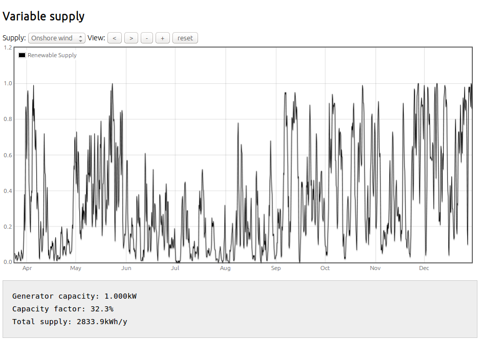
This example is useful for just seeing what the ZeroCarbonBritain renewable capacity factor dataset looks like, you can zoom and pan through the datasets for onshore wind, offshore wind, tidal, wave and solar pv, click on the link below to open the tool:
Online tool: http://openenergymonitor.org/energymodel > navigate to 1. variable supply
The units are really not important the example could just as well be in MW's or GW's. kW's where chosen as the other model examples in the series are focused around building a hourly model that's relatable to an average households energy demand. The kW's of installed capacity could just relate to a small share of a much larger wind turbine, solar farm, wave or tidal power installation.
Running the model for each of these generation types with the same installed capacity the results are as follows:
| Onshore wind | Offshore wind | Wave | Tidal | Solar | |
| Installed capacity | 1.0kW | 1.0kW | 1.0kW | 1.0kW | 1.0kW |
| Annual generation | 2834 kWh | 4204 kWh | 2482 kWh | 2092 kWh | 826 kWh |
| Capacity factor | 32% | 47% | 28% | 23% | 9% |
In all of the examples above the installed capacity of the renewable generator was the same (1.0kW) but we can see straight away that there is a significant difference in the total electricity generated by each type. A unit of offshore wind generates just over 5 times as much energy as a unit of solar pv using the zerocarbonbritain dataset. By itself this is not enough information to evaluate the effectiveness of a technology, we would need to compare the costs per unit of installed capacity, embodied energy per unit of installed capacity, how well a particular solution matches demand, the land areas required, the availability of the resource to name just a few of the many factors that need to be weighed up but it does highlight one of the important factors.
Python example source code
Alongside the online javascript modelling tool there are a series of python versions of the examples which are simpler to follow as they dont include all the code to create the visual output, they just print out the main results at the end.
The following 19 lines of python code are all you need to load the ZeroCarbonBritain dataset and run through all 87,648 hours, calculating the power output for each hour and accumulating the total energy supplied over the 10 year model period:
# dataset index:
# 0:onshore wind, 1:offshore wind, 2:wave, 3:tidal, 4:solar, 5:traditional electricity
gen_type = 4
installed_capacity = 1.0 # kW
# Load dataset
with open("../dataset/tenyearsdata.csv") as f:
content = f.readlines()
hours = len(content)
print "Total hours in dataset: "+str(hours)+" hours"
total_supply = 0
for hour in range(0, hours):
values = content[hour].split(",")
supply = float(values[gen_type]) * installed_capacity
total_supply += supply
capacity_factor = total_supply / (installed_capacity*hours) * 100
print "Installed capacity: %s kW" % installed_capacity
print "Total supply: %d kWh" % total_supply
print "Capacity factor: %0.2f%%" % capacity_factor
Next: Variable supply and flat demand - investigating the degree of supply/demand matching To engage in discussion regarding this post, please post on our Community Forum.